Follow these 4 steps to map out what areas are within 500m of a Bicycle share station and a bike shop. This tutorial is meant as an introduction to making static maps using ggmap, ggplot and R.
It would be convenient for people who live and work in these areas to see if they like biking (using the nearby share stations), and then invest in a bike of their own (purchase and upkeep from the nearby shop).
Codeschool’s Try R is an easy way to review syntax and learn basic operations. It runs in your browser so you do not need to download R or Rstudio to start learning.
1. Initial Setup
a) Load packages
In addition to the packages listed below, you will also need to have the raster package installed, however to not load this package.
library(tidyverse)
library(magrittr)
library(forcats)
library(jsonlite)
library(ggmap)
library(rgeos)
library(rgdal)
library(downloader)
library(ggpolypath)
Optionally, you can add a file.drawer path to permanently save maps once they are downloaded, and avoid repeatedly downloading the same map.
drawer.path <- "path_to_drawer"
b) Download and Import Data
# Station Locations
  station.locations.raw <- fromJSON("https://tor.publicbikesystem.net/ube/stations")

  station.locations <- station.locations.raw[[2]] %>%
    distinct(stationName, latitude, longitude) %>%
    set_colnames(c("name", "lat", "lon")) %>%
    mutate(id = "Share Station")

# Bike shops
  temp <- tempfile()
  temp2 <- tempfile()

  download.file("http://opendata.toronto.ca/gcc/bicycle_shop_wgs84.zip", temp)
  unzip(temp, exdir = temp2)
  shops.raw <- readOGR(dsn = temp2, layer = "BICYCLE_SHOP_WGS84")
  shops <- tibble(lat = shops.raw@data$LATITUDE,
                  lon = shops.raw@data$LONGITUDE,
                  id = "Retail Shop")

  unlink(temp)
  unlink(temp2)
2. Plot bicycle share stations
a) Download base map
We can use the ggmap package to get a snapshot of a google map which we will use as our base map. We can customize the style of the google map using the style argument in the get_googlemap() function. You can create the style arguments interactiverly using the Google Maps API styling Wizard.
  # Map Area
  zoom <- 12
  avg.coords <- c(-79.39,43.67)
  options(ggmap.file_drawer =  drawer.path)

  # Map Style
  style <-  "feature:poi.attraction%7Celement:labels%7Cvisibility:off&style=feature:poi.business%7Celement:labels%7Cvisibility:off&style=feature:poi.government%7Celement:labels%7Cvisibility:off&style=feature:poi.medical%7Celement:labels%7Cvisibility:off&style=feature:poi.park%7Celement:labels%7Cvisibility:off&style=feature:poi.place_of_worship%7Celement:labels%7Cvisibility:off&style=feature:poi.school%7Celement:labels%7Cvisibility:off&style=feature:poi.sports_complex%7Celement:labels%7Cvisibility:off&size=480x360"

  # Download Map
  raw.map <- get_googlemap(center = avg.coords,
                         maptype = "roadmap",
                         archiving = T,
                         zoom = zoom,
                         style = style)

  base.map <- ggmap(raw.map)

base.map

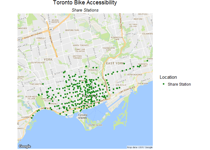
b) Add share station location to map
Once we have the base map layer, we can add points onto the map the same way we would create any scatter plot. We can add titles and adjust the plot style using a list of plot theme objects.
  # Station locations

    plot.stations <- geom_point(data = station.locations, aes(y = lat, x = lon, colour = id))

  # Aesthetics of maps
    map.theme <- list(theme_void(),
                      theme(plot.title = element_text(hjust = 0.5),
                            plot.subtitle = element_text(hjust = 0.5, face = "italic"),
                            plot.caption = element_text(hjust = 0, size = 6)),
                      scale_colour_manual(values = c("forestgreen", "blue")))
  # Map 1
    base.map +
      plot.stations +
      map.theme +
      labs(title = "Toronto Bike Accessibility",
           subtitle = "Share Stations",
           colour = "Location")
3. Highlight area around stations
We define three functions to tackle this part of the task. 1. get_map_edges() lets us know the edges of the map. We will need this to cut off polygons at the edge. 2. get_circle() takes each point and uses the gBuffer() function to project the point outward 500m, creating a polygon. 3. plot_polygon() takes a raw polygon and converts it into a geom_polygon which we can add to our map.
  # Get edges of the map

    get_map_edges <- function(map){

      attr(map, "bb") %>%
        as.list() %>%
        set_names(c("y.min", "x.min", "y.max", "x.max"))

    }

    map.edges <- get_map_edges(raw.map)

  # Draw Circles

    get_circle <- function(coordinates, radius, map.edges){

      spatial <- SpatialPointsDataFrame(coords = coordinates %>% select(lon, lat),
                                        data = coordinates %>% select(lon, lat),
                                        proj4string=CRS("+proj=longlat +ellps=WGS84 +datum=WGS84"))

      gnom <- sprintf("+proj=gnom +lat_0=%s +lon_0=%s +x_0=0 +y_0=0",
                      spatial@coords[1,][[2]], spatial@coords[1,][[1]])
      spatial.circles <- spTransform(spatial, CRS(gnom))

      circles <- suppressWarnings(gBuffer(spatial.circles, byid = TRUE, width = radius, quadsegs = 15)) %>%
        spTransform(., CRS("+init=epsg:4326"))

      return(circles)
    }

    circles.stations.raw <- station.locations %>%
      get_circle(500, map.edges) %>%
      raster::aggregate()

    plot_polygon <- function(polygon, map.edges, colour.x, alpha = 0.05){
      polygon %>%
        fortify() %>%
        mutate(long = pmax(map.edges$x.min, pmin(map.edges$x.max, long)),
               lat = pmax(map.edges$y.min, pmin(map.edges$y.max, lat))) %>%
        geom_polypath(data = ., aes(x = long, y = lat, group=group), color = colour.x, fill = colour.x, alpha = 0.05)
    }

    circles.stations <- circles.stations.raw %>%
      plot_polygon(map.edges, "forestgreen")

    # Map 1
    base.map +
      plot.stations +
      circles.stations +
      map.theme +
      labs(title = "Toronto Bike Accessibility",
           subtitle = "Share Stations Service Area",
           caption = "[1] Service area is within 500m.",
           colour = "Location")

4. Get overlap areas
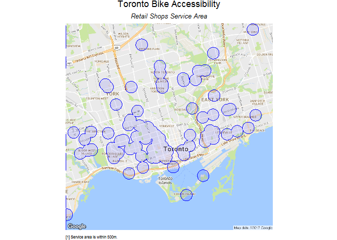
a) Service area around shops
Using the shop locations we downloaded from Open Toronto we can get the 500m service area of each shop. It would be easy to bring your bike in for repairs and tune-ups if you lived within 500m of a shop.
  # Draw Circles

    circles.shops.raw <- shops %>%
      get_circle(500, map.edges) %>%
      raster::aggregate()

    circles.shops <- circles.shops.raw %>%
      plot_polygon(map.edges, "blue")

  # Map 1
    base.map +
      circles.shops +
      circles.shops +
      map.theme +
      labs(title = "Toronto Bike Accessibility",
           subtitle = "Retail Shops Service Area",
           caption = "[1] Service area is within 500m.",
           colour = "Location")
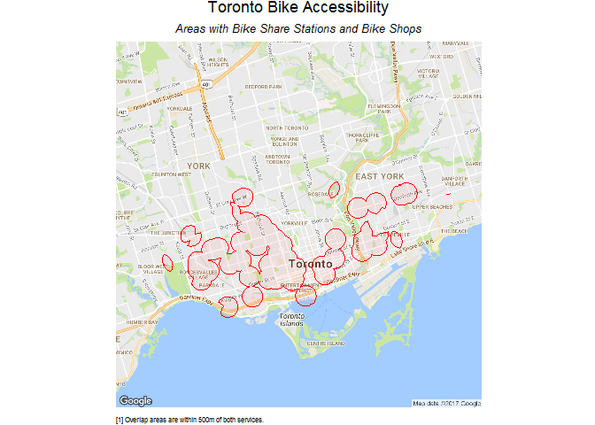
b) Overlap Areas
We can use the raster::intersect() function to get a polygon of the overlap area between the shop service area and the share stations. Remeber not to load the raster package as it will have conflicts with other packages we have loaded.
  overlap.area.raw <- raster::intersect(circles.shops.raw, circles.stations.raw)

  overlap.area <- overlap.area.raw %>%
    plot_polygon(map.edges, "red")

  base.map +
    overlap.area +
    map.theme +
    labs(title = "Toronto Bike Accessibility",
         subtitle = "Areas with Bike Share Stations and Bike Shops",
         caption = "[1] Overlap areas are within 500m of both services.")
That’s it!