Follow these 4 steps to create probability based contour maps in R. You will need to download R and RStudio. Even relatively inexperienced R users should be able to follow along.
Codeschool’s Try R is an easy way to review syntax and learn basic operations. It runs in your browser so you do not need to download R or Rstudio to start learning.
1. Setup
a) Load packages
You may first need to install a package if you have not already done so. To install a package use the install.packages() function. For example, to install the tidyverse package run install.packages("tidyverse"). Notice how the package name is inside quotes.
Once you have installed the packages, run the following chunk of code. You can run the chunk by clicking the Run button.
library(readxl)
library(rgdal)
library(tidyverse)
library(ks)
library(ggmap)
library(magrittr)
library(stringr)
library(rgeos)
Optionally, you can add a file.drawer path to permanently save maps once they are downloaded, and avoid repeatedly downloading the same map.
drawer.path <- "path_to_drawer"
b) Download and Import the Data
Download a .zip of fire station locations data from the City of Toronto’s open data site and saved it in a temp file. Open the zip file and load in the .xls of fire station locations.
fire_data_link <- "https://www1.toronto.ca/City_Of_Toronto/Information_Technology/Open_Data/Data_Sets/Assets/Files/fire_stns.zip"
temp <- tempfile()
temp2 <- tempfile()

download.file(fire_data_link, temp)
unzip(zipfile = temp, exdir = temp2)
fires.raw <- read_xls(file.path(temp2, "fire station x_y.xls"), col_names = c("stn.num", "x", "y"))

unlink(c(temp, temp2))
rm(temp, temp2)
2. Convert coordinate system
Converting from UTM system to a lat & lon system. Notice the CRS projection specifies the appropriate zone +zone=17.
fires.raw.sp <- SpatialPoints(fires.raw %>% select(x, y), proj4string=CRS("+proj=utm +zone=17 +datum=WGS84"))
fires.sp <- spTransform(fires.raw.sp, CRS("+proj=longlat +datum=WGS84"))

fires <- as.data.frame(fires.sp) %>%
  set_colnames(c("lon", "lat"))
3. Initial Maps
a) Download Map
Use make\_bbox to calculate the bounding box of our fire stations data. We use f = 0.3 to add padding to the box. We then calculate the zoom need to get a map which contains all points in the bounding box. Use get_googlemap to download the underlying map image. Set archiving = T to avoid downloading the map multiple times. If you want to remember your map download across sessions set the global option for ggmap.file_drawer.
bbox <- make_bbox(lon = lon, lat = lat, data = fires, f = 0.3)
zoom <- calc_zoom(lon = bbox)

avg.coords <- bbox %>%
  as.list() %$%
  c(mean(c(left, right)),
    mean(c(top, bottom)))

options(ggmap.file_drawer =  drawer.path)

to.map <- get_googlemap(center = avg.coords,
                        maptype = "roadmap",
                        archiving = T,
                        zoom = zoom)
b) Set Plot Aesthetics
Create and object to specify the aesthetics for the plot. This specifies things such as font sizes, tick marks, title alignment etc. To learn more about plot aesthetics see the ggplot site
plot.theme <- theme(plot.title = element_text(hjust = 0.5),
                    plot.subtitle = element_text(hjust = 0.5, face = "italic"),
                    plot.margin=unit(c(0.5,0.5,2,0.5),"cm"),
                    plot.caption = element_text(hjust = 0, size = 6),
                    axis.title.x=element_blank(),
                    axis.text.x=element_blank(),
                    axis.ticks.x=element_blank(),
                    axis.title.y=element_blank(),
                    axis.text.y=element_blank(),
                    axis.ticks.y=element_blank(),
                    legend.text=element_text(size=8))
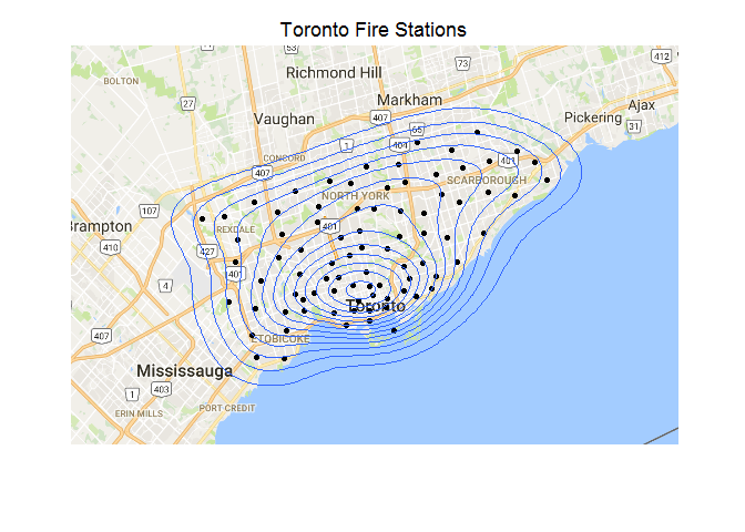
c) Create the initial plot
Use the stat_density_2d function to plot some initial contours.
ggmap(to.map) +
  geom_point(data = fires, aes(x = lon, y = lat)) +
  ylim(as.list(bbox)$bottom, as.list(bbox)$top) +
  xlim(as.list(bbox)$left, as.list(bbox)$right) +
  stat_density_2d(data = fires) +
  labs(title = "Toronto Fire Stations") +
  plot.theme
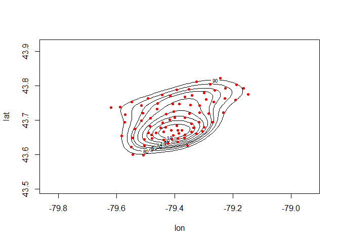
4. Draw a specific contour
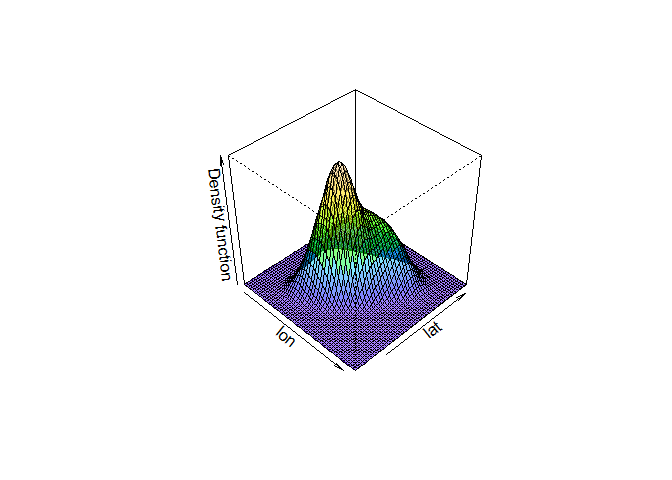
Use the kde function from the ks package to calculate contours which encircle a specific % of the fire stations. We can do some basic plots to see the kernel densities. We will also draw a contour around 50% of the stations.
fires.mat <- fires %>% select(lon, lat)

fires.kde <- kde(x = fires.mat, binned=TRUE)

p1 <- plot(fires.kde, cont = 1:9 * 10)
points(fires$lon, fires$lat, pch = 20, col = "red")
plot(fires.kde, display = "persp", theta = 45)
contour.level <- 50
contour.spec <- str_c(100 - contour.level, "%")

contour.x1 <- with(fires.kde, contourLines(x=eval.points[[1]], y=eval.points[[2]],
                                    z=estimate, levels=cont[contour.spec])[[1]])
contour.x <- data.frame(contour.x1)

ggmap(to.map) +
  geom_point(data = fires, aes(x = lon, y = lat)) +
  ylim(as.list(bbox)$bottom, as.list(bbox)$top) +
  xlim(as.list(bbox)$left, as.list(bbox)$right) +
  geom_path(aes(x, y), data=contour.x, colour = "red", size = 1) +
  labs(title = "Toronto Fire Stations",
       subtitle = "50% Contour") +
  plot.theme
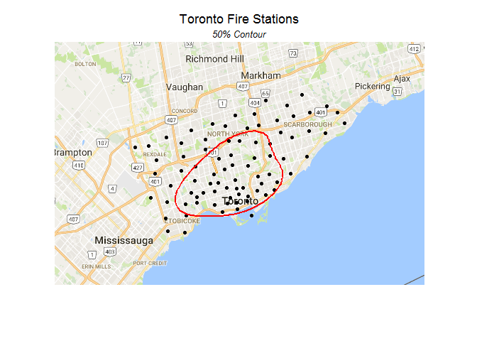
We can then use the gContains function to check which stations fall within the contour and calculate the exact share.
fires.sp <- SpatialPoints(fires.mat, proj4string = CRS("+init=epsg:4326"))

contour.x.sp <- contour.x %>%
  mutate(id = 1) %>%
  select(id, x, y) %>%
  group_by(id) %>%
  do(poly= dplyr::select(., x, y) %>%Polygon()) %>%
  rowwise() %>%
  do(polys=Polygons(list(.$poly),.$id)) %>%
  {SpatialPolygons(.$polys, proj4string = CRS("+init=epsg:4326"))} %>%
  SpatialPolygonsDataFrame(data.frame(data = 1, row.names = 1))

in.contour <- gContains(contour.x.sp, fires.sp, byid = T)
sum(in.contour)
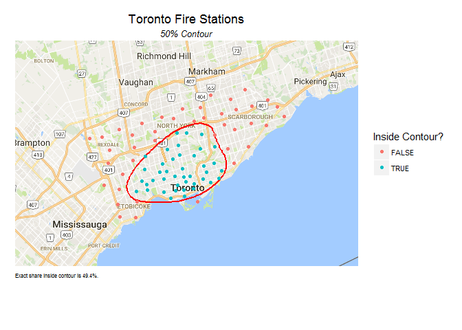
We see 41 of the 83 sites are within the 50% contour.
## [1] 41
ggmap(to.map) +
  geom_path(aes(x, y), data=contour.x, colour = "red", size = 1) +
  geom_point(data = fires, aes(x = lon, y = lat, colour = in.contour)) +
  ylim(as.list(bbox)$bottom, as.list(bbox)$top) +
  xlim(as.list(bbox)$left, as.list(bbox)$right) +
  labs(title = "Toronto Fire Stations",
       subtitle = "50% Contour",
       colour = "Inside Contour?",
       caption = str_c("Exact share inside contour is ", round(sum(in.contour)/nrow(fires) * 100, 1), "%.")) +
  plot.theme
5. Draw specific contour function
This is a general purpose function for drawing a series of contours and adding them to a map plot. It takes three arguments; 1) the contour levels to plot as a numeric vector (eg. 20, 30, ..), the data of points as a matrix of lat and lons, and a kde object (the output of the kde function).
The function return nested list with an element for each contour level. Each element is list of length 2. The first “polygon” element contains a dataframe specifying the polygon of the contour. The second “exact.share” element contains the share of points contained within the contour.
add_contour_x <- function(contour.level, data, kde.obj){

  # Data matrix with lon and lats

  contour.spec <- str_c(100 - contour.level, "%")
  contour.x1 <- with(kde.obj, contourLines(x=eval.points[[1]], y=eval.points[[2]],
                                             z=estimate, levels=cont[contour.spec])[[1]])
  contour.x <- data.frame(contour.x1)

    # Check the exact share inside the contour and add a note

    data.sp <- SpatialPoints(data, proj4string = CRS("+init=epsg:4326"))

  contour.x.sp <- contour.x %>%
    mutate(id = 1) %>%
    select(id, x, y) %>%
    group_by(id) %>%
    do(poly= dplyr::select(., x, y) %>% Polygon()) %>%
    rowwise() %>%
    do(polys=Polygons(list(.$poly),.$id)) %>%
    {SpatialPolygons(.$polys, proj4string = CRS("+init=epsg:4326"))} %>%
    SpatialPolygonsDataFrame(data.frame(data = 1, row.names = 1))

  in.contour <- gContains(contour.x.sp, data.sp, byid = T)

  # Outputs
  exact.share <- sum(in.contour) / length(in.contour)

  return(list(polygon = contour.x,
              exact.share = exact.share))

}
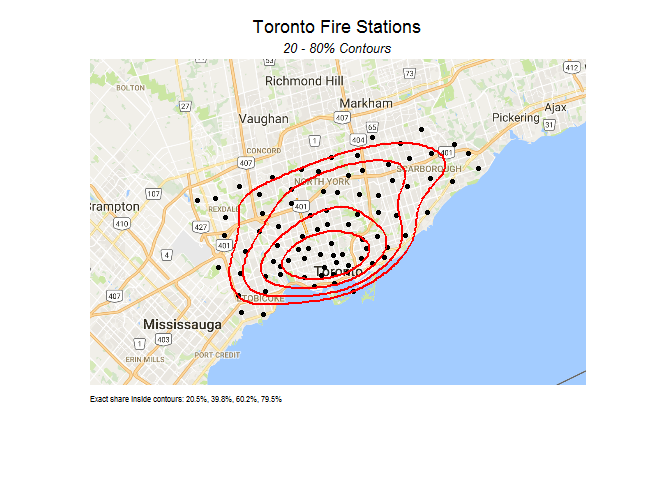
Here we use the function to create 20, 40, 60 and 80% contours. We then use the polygon elements output to create geom_path layers (the contour polygons) to add to the map. We use the “exact.share” elements to create the footnotes for the map.
add.contours.out <- c(1:4 * 20) %>%
  map(add_contour_x, data = fires.mat, kde.obj = fires.kde)


all.contours <- add.contours.out %>%
  map("polygon") %>%
  map( ~ geom_path(aes(x, y), data = ., colour = "red", size = 1))

notes <- add.contours.out %>%
  map_dbl("exact.share") %>%
  round(., 3) %>%
  `*`(100) %>%
  str_c("%", collapse = ", ") %>%
  str_c("Exact share inside contours: ", .)

ggmap(to.map) +
  geom_point(data = fires, aes(x = lon, y = lat)) +
  ylim(as.list(bbox)$bottom, as.list(bbox)$top) +
  xlim(as.list(bbox)$left, as.list(bbox)$right) +
  all.contours +
  labs(title = "Toronto Fire Stations",
       subtitle = "20 - 80% Contours",
       caption = notes) +
  plot.theme
That’s it. Done!